HashTables

What is a Hash Table §

A hash table is a data structure that uses an array to store key-value pairs. It uses a hash function that computes an index of the array when given a key.

What is a hash function §

A hash function is a function to map data to a fixed sized value. In this case we are using the hash function to index a fixed size array.

• A hash function should be relatively cheap to compute
• Deterministic. Given the same key, it will always return the same number
• Ideally, maps keys uniformly over the range of indices

Usually the modulo operator ’%’ is used as the last step in the hash function as it conveniently maps to the range of indices.

For example for an array of size 11 and the array [ 4,8,15,16,23,42 ]:

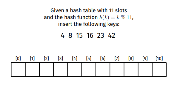
4 would be inserted at index $4\%11=4$ 8 would be inserted at index $8\%11=8$ 15 would be inserted at index $15\%11=4$

But since 4 is already in index [ 4 ] then we cannot place 15 in the same index. This is known as a hash collision.

There are three common methods of resolving hash collisions

• Separate Chaining
• Linear Probing
• Double Hashing

Separate Chaining §

Separate chaining involves using an array of linked lists instead of just an array of values. Each node of the linked list contains both the key and value. When a hash collision occurs then we traverse the linked list until the key we are looking for matches the key in a linked list node.

For a hash table with $N$ array slots and $M$ items, then the average length of the linked lists in the table would be $M/N$. Therefore the average operation cost would be $O(M/N)$, worst case all the items would be in the same index meaning $O(M)$.

To avoid degrading performance the hash table should be resized when $M/N\approx 1$

Linear Probing §

Linear probing does not involve introducing another data structure to store the collisions. Instead we linearly search the next slot until an empty slot is found.

On lookup/insertion the key is hashed to get an index. From that index if the item in the slot does not have the same key then we go to the next one and so on until the keys match.

Doing this means deletions are not straight forward. Backshift This method is the brute force method for deletion. After deleting check the next slot, if the slot is not empty then re-insert that item. Continue doing this until an empty slot is encountered.

Tombstone (Lazy Deletion) Replace the deleted item with a “Deleted” marker (AKA a tombstone). The tombstone is treated as empty for insertions and treated as occupied during lookup. Being treated as occupied for lookup is important so that items can still be linearly searched, if it was treated as empty then it may not be possible for the linear search to find a matching key.

Problems with Linear Probing §

Clustering is a problem for linear probing. Clustering is where data is inserted continuously due to many items with a similar index after hashing. If a cluster is long enough then subsequent insertions may already be within a cluster and the cluster size would continue to increase. Long clusters means insertions and lookups may need to traverse the entire length of a hash table to find/insert the correct item.

Quadratic probing is a variant of linear probing which use a quadratically increasing step size. E.g if the hashed index is x then it will search the indexes $x+1$, $x+4$, $x+9$, $x+16$, $x+25$ and so on until an empty slot is found. This can result in secondary clustering where the clustering only occurs when the two keys result in the same initial hash which is less severe in terms of performance but clustering can still occur.

Double Hashing §

Double Hashing is similar to linear probing except instead of just searching for the next empty slot it uses a step size increment based on hashing the key a second time. Using an offset based on the second hash is to minimise clustering.

The second hash needs to be well designed to ensure that it can visit all slots so it can never return $0$. A popular second hashing function can be described as follows: $h_2(key)=primeNum\pm (key\%primeNum)$

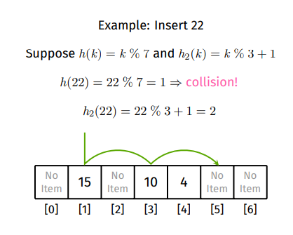In this example

1. $h_1(22)=1$ . Since index 1 is occupied then secondary hash is required to get offset.
2. $h_2(22)=2$. Offset is 2, $1+2=3$, index 3 is occupied so then calculate the next step.
3. Offset is 2, $3+2=5$, index 5 is empty so insert into index 5.

The hash table size also needs to be a prime number to ensure all slots can be visited. Even with a bad secondary hash it will eventually search all indexes

For example if you had a table of size 15 (non-prime) and the keys [15,30,45,60]. If $h_1(key)=(key\%tableSize)$ and for some reason the secondary hash always returned 5, $h_2(key)=5$ then the results would be:

1. $h_1(15)=0$ . Since index 0 is empty then insert at index 0.
2. $h_1(30)=0$ . Since index 0 is occupied then hash again to get offset. a. $h_2(30)=5$. Offset is 5, 0+5 = 5, index 5 is empty then insert at index 5.
3. $h_1(45)=0$ . Since index 0 is occupied then hash again. a. $h_2(45)=5$. Offset is 5, 0+5 = 5, index 5 is also occupied so increment by offset again to index 10. Index 10 is empty so insert at index 10.
4. $h_1(60)=0$ . Since index 0 is occupied then hash again. With the same logic the offset will be 5. Since the table is size 15 the largest index is 14. When the offset reaches the length of the table then it wraps back around to the start which is 0. And since index 0,5 and 10 are occupied, we will get stuck in a loop searching for an empty spot.

Now if we try using a table of size 13 (prime number) and the keys[13,26,39,52] with the same hashing functions.

1. $h_1(13)=0$ . Since index 0 is empty then insert at index 0.
2. $h_1(26)=0$ . Since index 0 is occupied then hash again to get offset. a. $h_2(26)=5$. Offset is 5, 0+5 = 5, index 5 is empty then insert at index 5.
3. $h_1(39)=0$ . Since index 0 is occupied then hash again. a. $h_2(39)=5$. Offset is 5, 0+5 = 5, index 5 is also occupied so increment by offset again to index 10. Index 10 is empty so insert at index 10.
4. $h_1(52)=0$ . Since index 0 is occupied then hash again. With the same logic the offset will be 5. Since the table is size 13 the largest index is 12. Since 10+5 =15 is bigger than the length of the table then we wrap back to the start and will be inserting at index 2.
5. If the keys contained more multiples of 13 then the inserted indexes would be [0, 5, 10, 2, 7, 12, 4, 9, 1, 6, 11, 3] and so on.

For deletion operations the methods still are the same as linear probing. Back shifting is more difficult to compute so Tombstone deletion is preferred.

Hash Table Resizing §

The initial size of a hash table has trade offs. Allocating a high initial size means a large amount of memory needs to be allocated. If a low initial size is used and there are many items then the hash table will need to be continuously resized.

Since the underlying data structure of a hash table is an array, to increase the size we would need to allocated a new array that is approximately two times larger and then rehash all the values in the original table to the new larger table. Hence resizing a lot can be expensive.

Hash tables automatically resize when they get too full. But what is the threshold for too full? The load factor is the ratio of how many items are in the table compared to the size of the table, $\alpha =M/N$ where $M$ is the number of items and $N$ is the size of the table.

The default load factor for the implementation of hash tables in C++ and Java use 0.75. The default load factor of 0.75 is described to offer a good trade off between time and space costs. A higher load factor would mean the table is more full, less space is utilised but more collisions would occur. A lower load factor would mean the table is more empty, collisions would be less likely and space needs to be overallocated.

References §

• Hashing - UT Computer Science
• COMP2521 - UNSW
• Hash Table - Oracle