CPU Scheduling

CPU Scheduling §

We have yet to understand the high-level policies that an OS scheduler employs. We will now do just that, presenting a series of scheduling policies (sometimes called disciplines) that various smart and hard-working people have developed over the years. Let us first make a number of simplifying assumptions about the processes running in the system, sometimes collectively called the workload. Determining the workload is a critical part of building policies, and the more you know about workload, the more fine-tuned your policy can be

Lets start with these unrealistic assumptions

1. Each job runs for the same amount of time.
2. All jobs arrive at the same time.
3. Once started, each job runs to completion.
4. All jobs only use the CPU (i.e., they perform no I/O)
5. The run-time of each job is known.

Scheduling Metrics The turnaround time of a job is defined as the time at which the job completes minus the time at which the job arrived in the system. More formally, the turnaround time is: $T_{turnaround}=T_{completion}-T_{arrival}$

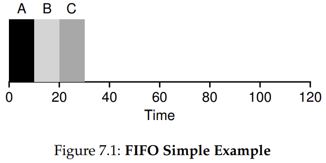
First In - First Out (FIFO) §

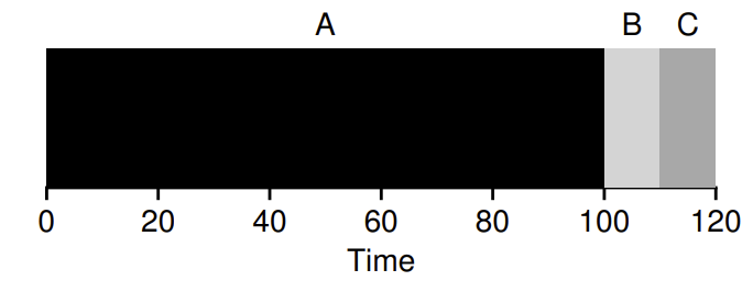
Imagine three jobs arrive in the system, A, B, and C, at roughly the same time ($T_{arrival}=0$). Because FIFO has to put some job first, let’s assume that while they all arrived simultaneously, A arrived just a hair before B which arrived just a hair before C. Assume also that each job runs for 10 seconds. What will the average turnaround time be for these jobs? 20 seconds.

But if we relax assumption 1 and that each job does not run for the same time then the the resulting turnaround time is much higher. $\frac{100+110+120}{3}=110$

Shortest Job First (SJF) §

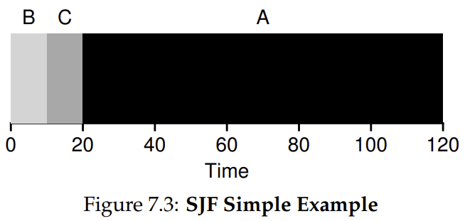By running the shortest jobs first we can achieve a much better turnaround $\frac{10+20+120}{3}=50$ However if you relax assumption 2 and $A$ arrives at $t=0$, $B$ arrives at $t=10$ and $C$ arrives at $t=20$ then we would end up with the same issue of A executing first and blocking the subsequent jobs even though they are much shorter

Shortest Time to Completion First (STCF) §

If we relax assumption 3 that all jobs must run to completion then the scheduler can context switch to the shortest jobs when they arrive. 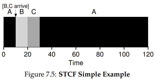At any time the scheduler receives a new job the scheduler determines which remaining jobs have the least time left. $\frac{120+(20-10)+(30-20)}{3}=50$

Response Time §

Thus, if we knew job lengths, and that jobs only used the CPU, and our only metric was turnaround time, STCF would be a great policy. In fact, for a number of early batch computing systems, these types of scheduling algorithms made some sense. However, the introduction of time-shared machines changed all that. Now users would sit at a terminal and demand interactive performance from the system as well. And thus, a new metric was born: response time.

$T_{response}=T_{firstrun}-T_{arrival}$

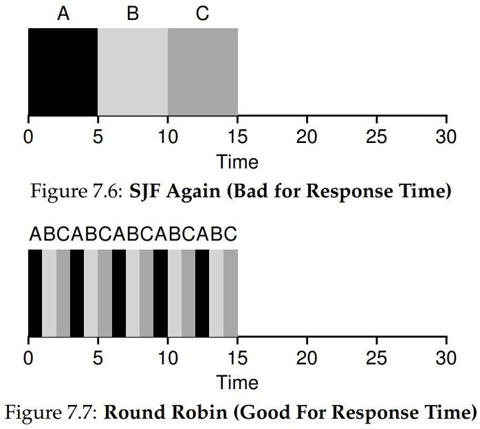
STCF and related disciplines are not particularly good for response time. If three jobs arrive at the same time, for example, the third job has to wait for the previous two jobs to run in their entirety before being scheduled just once. While great for turnaround time, this approach is quite bad for response time and interactivity. Indeed, imagine sitting at a terminal, typing, and having to wait 10 seconds to see a response from the system just because some other job got scheduled in front of yours. How can we build a scheduler that is sensitive to response time?

Round Robin (RR) §

Instead of running jobs to completion, RR runs a job for a time slice and then switches to the next job in the run queue. It repeatedly does so until the jobs are finished. For this reason, RR is sometimes called time-slicing

• The shorter the time slice, the better the performance of RR under the response-time metric.
  • However, making the time slice too short is problematic: suddenly the cost of context switching will dominate overall performance.
  • Length of the time slice presents a trade-off to a system designer, making it long enough to amortize the cost of switching without making it so long that the system is no longer responsive.

RR is indeed one of the worst policies if turnaround time is our metric.

• RR is stretching out each job as long as it can, by only running each job for a short bit before moving to the next.
• Turnaround time only cares about when jobs finish, RR is nearly pessimal, even worse than simple FIFO in many cases.

More generally, any policy (such as RR) that is fair, i.e., that evenly divides the CPU among active processes on a small time scale, will perform poorly on metrics such as turnaround time. Indeed, this is an inherent trade-off: if you are willing to be unfair, you can run shorter jobs to completion, but at the cost of response time; if you instead value fairness,

• Trade off response time vs fairness

Incorporating I/O §

When a job initiates an I/O request it is blocked waiting for I/O completion.

Scheduler should execute a different job on the CPU while the current job is blocked. Once the I/O is complete should the CPU

• Move the process that issued the I/O from blocked to ready
• Run the process when I/O is complete

Example: A runs for 10 ms and then issues an I/O request (assume here that I/Os each take 10 ms), B uses the CPU for 50 ms and performs no I/O. The scheduler runs A first, then B after. Assume we are trying to build a STCF scheduler. How should such a scheduler account for the fact that A is broken up into 5 10-ms sub-jobs,

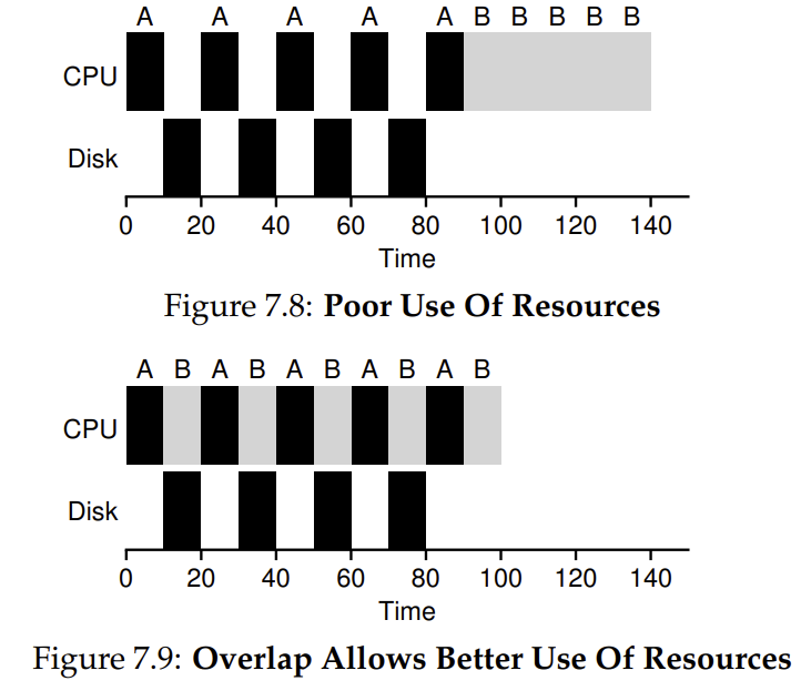
A common approach is to treat each 10-ms sub-job of A as an independent job. Thus, when the system starts, its choice is whether to schedule a 10-ms A or a 50-ms B. With STCF, the choice is clear: choose the shorter one, in this case A

Multi Level Feedback Queue (MLFQ) §

The worst assumption is that the OS knows the length of each job. Usually the OS knows very little about the length of each job. Thus, how can we build an approach that behaves like SJF/STCF to optimise turnaround time without such a priori knowledge? Further, how can we incorporate some of the ideas we have seen with the RR scheduler so that response time is also quite good? The MLFQ tries to address these problems.

Rules §

The MLFQ has a number of distinct queues, each assigned a different priority level. At any given time, a job that is ready to run is on a single queue. MLFQ uses priorities to decide which job should run at a given time: a job with higher priority (i.e., a job on a higher queue) is chosen to run. More than one job may be on a given queue, and thus have the same priority. In this case, we will just use round-robin scheduling among those jobs.

• Rule 1: If Priority(A) > Priority(B), A runs (B doesn’t).
• Rule 2: If Priority(A) = Priority(B), A & B run in RR.

The key to MLFQ scheduling therefore lies in how the scheduler sets priorities. Rather than giving a fixed priority to each job, MLFQ varies the priority of a job based on its observed behaviour.

• If a job repeatedly relinquishes the CPU while waiting for input from the keyboard, MLFQ will keep its priority high, as this is how an interactive process might behave.
• If a job uses the CPU intensively for long periods of time, MLFQ will reduce its priority.

The problem with just these rules is if the CPU continuously receives interactive processes then they will monopolise CPU time and thus long running jobs will never receive any CPU time. To solve this we may just set all incomplete jobs to the highest priority after some time period $S$. If it is set too high, long-running jobs could starve; too low, and interactive jobs may not get a proper share of the CPU.

Another issue is that CPU time can be gamed by issuing an I/O operation right before the allotment time is used up to retain the priority. To solve this the scheduler needs to refine the previous rule:

• Once a job uses up its time allotment at a given level (regardless of how many times it has given up the CPU), its priority is reduced (i.e., it moves down one queue).

Lottery Scheduling §

Tickets are used to represent the share of a resource that a process should receive. The percent of tickets that a process has represents its share of the system resource in question. The goal is to achieve fairness in scheduling.

Imagine two processes, A and B, and further that A has 75 tickets while B has only 25. Thus, what we would like is for A to receive 75% of the CPU and B the remaining 25% Lottery scheduling achieves this probabilistically (but not deterministically) by holding a lottery every so often (say, every time slice). Holding a lottery is straightforward: the scheduler must know how many total tickets there are (in our example, there are 100). The scheduler then picks a winning ticket from 0-99. Assuming A holds tickets 0 through 74 and B 75 through 99, the winning ticket simply determines whether A or B runs.

Ticket Mechanisms §

Ticket Currency

• User can allocate tickets in their own jobs in whatever currency they like. System can then convert these to the global value.
  • User A is allocated 100 Global tickets and has two jobs A1 and A2
  • A1 is allocated 500 A tickets and A2 is allocated 500 A tickets
  • The system can then convert these to A1 and A2 with 50 Global tickets each

Ticket Transfer

• A process can temporarily hand off its tickets to another process

This ability is especially useful in a client/server setting, where a client process sends a message to a server asking it to do some work on the client’s behalf. To speed up the work, the client can pass the tickets to the server and thus try to maximize the performance of the server while the server is handling the client’s request. When finished, the server then transfers the tickets back to the client and all is as before.

Ticket Inflation

• A process can temporarily raise or lower the number of tickets it owns.
• If any one process knows it needs more CPU time, it can boost its ticket value as a way to reflect that need to the system, all without communicating with any other processes.
  • In a competitive scenario with processes that do not trust one another, this makes little sense; one greedy process could take over the machine.

The Linux Completely Fair Scheduler (CFS) §

Whereas most schedulers are based around the concept of a fixed time slice, CFS operates a bit differently. Its goal is simple: to fairly divide a CPU evenly among all competing processes. It does so through a simple counting-based technique known as virtual runtime (vruntime).

Each process’s vruntime increases at the same rate, in proportion with physical (real) time. When a scheduling decision occurs, CFS will pick the process with the lowest vruntime to run next.

• if CFS switches too often, fairness is increased, as CFS will ensure that each process receives its share of CPU even over miniscule time windows, but at the cost of performance (too much context switching);
• if CFS switches less often, performance is increased (reduced context switching), but at the cost of near-term fairness

CFS manages this tradeoff through various parameters sched_latency

• A value to determine how long one process should run before considering a switch
  • Calculate the time slice by dividing the sched_latency value by the number of processes
• Typical value is 48 milliseconds

$\text{time slice}=\text{sched\_latency}/n$ However when $n$ is large then the time slice would become too small and the context switching overhead will reduce performance

min_granularity

• The minimum length of time a time slice can be.
• Typical value is about 6 milliseconds

e.g if you have 12 processes then for a sched_latency of 48ms then the time slice length would be 4ms. This is below the minimum granularity. The minimum granularity will ensure high CPU efficiency but wont be perfectly fair.

Niceness (Weighting/Priority) §

CFS also enables controls over process priority, enabling users or administrators to give some processes a higher share of the CPU.

It does this through a UNIX mechanism known as the nice level of a process. The nice parameter can be set anywhere from -20 to +19 for a process, with a default of 0.

Positive nice values imply lower priority and negative values imply higher priority.

Niceness can be factored in to compute the time slice length. ${\text{time\_slice}}_k=\frac{{\text{weight}}_k}{{\sum }_{i=0}^{n-1}{\text{weight}}_i}\cdot \text{sched\_latency}$ In addition to generalizing the time slice calculation, the way CFS calculates vruntime must also be adapted. Here is the new formula, which takes the actual run time that process j has accrued and scales it inversely by the weight of the process,

${\text{vruntime}}_j={\text{vruntime}}_j+\frac{{\text{weight}}_0}{{\text{weight}}_j}\cdot {\text{runtime}}_j$

References §

• OSTEP
  • (Havent included Chapter 10 yet)